The Levenberg-Marquardt algorithms solves the problem to minimize |f(v)| in the Euclidean norm, where f maps n variables to m variables, and n<=m. For linear f, we have to minimize |Ax-b|, which is simply a linear fit, and can be solved using various functions in Euler (fit, fitnormal, svdsolve).
The idea of the algorithm is to linearize f using the Jacobian derivative matrix. In each step, we minimize |f(a)+Df(a).(x-a)| for x. For n=m this is precisely the Newton method.
However, the problem can also be solves with Nelder-Mead. This notebook compares inplementations of the two methods in Euler.
Let us assume the following function.
>expr &= [x^2+y^2-1,x*y-1,x+2*y+1]
                   2    2
                 [y  + x  - 1, x y - 1, 2 y + x + 1]
We make it a function of x and y, which can also be used for row vectors.
>function f([x,y]) &= expr
                   2    2
                 [y  + x  - 1, x y - 1, 2 y + x + 1]
For the Nelder-Mead method, we need a function mapping vectors to reals.
>function fh([x,y]) := norm(f([x,y]))
Let us plot this function. The minimum is clearly visible.
>plot2d("fh",r=2,contour=1):
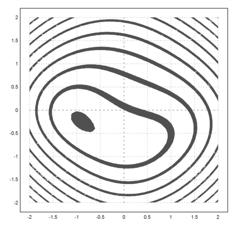
The Nelder-Mead method solves this minimization problem easily.
>v=nelder("fh",[0,0]), fh(v)
[-0.913985,  -0.235233]
0.880894013725
Now, for the Levenberg-Marquard algorithm, we need the Jacobian. We let Maxima compute that for us.
>function Df([x,y]) &= jacobian(@expr,[x,y])
                             [ 2 x  2 y ]
                             [          ]
                             [  y    x  ]
                             [          ]
                             [  1    2  ]
The following is a very simple implementation of the Levenberg-Marquard algorithm.
The function nlfit (non linear fit) needs two functions and a start vector. The first function f(v) must work for row 1xn vectors v, and produce a 1xm row vector as its result. The second function Df(v) must also work on row vectors, but produce an mxn Jacobian.
>help nlfit
nlfit is an Euler function.

function nlfit (f$, Df$, v)

Function in file : numerical

Minimizes f(x) from start vector v.

This method is named after Levenberg-Marquardt. It minimizes a
function from n variables to m variables (m>n) by minimizing the
linear tangent function. If the norm gets larger it decreases the
step size, until the step size gets closer than epsilon.

f(x) maps 1xn vectors to 1xm vectors (m>n)
Df(x) is the Jacobian of f.

>function f([x,y]) &= [x,y,x^2+2*y^2+1];
>function Df([x,y]) &= jacobian(f(x,y),[x,y]);
>nlfit("f","Df",[0.2,0.1])
 [-9.19403e-011,  -1.07327e-010]
>function h(v) := norm(f(v))
>nelder("h",[3,1]) // for comparison
 [6.33484e-007,  -1.9733e-007]
It works well, even for start vectors, which are not close to the optimal solution.
>v=nlfit("f","Df",[1,0]), fh(v)
[-0.913985,  -0.235232]
0.880894013725
I want to try another example, a non-linear quadratic approximation.
For a non-linear class of approximating functions we take the following rational functions. The problem with this class is that |c| must not be larger than 1 to avoid poles in the approximation interval [-1,1].
>fexpr &= (a*x+b)/(1+c*x)
                               a x + b
                               -------
                               c x + 1
We approximate exp(x) on discrete points.
>xv=-1:0.1:1; yv=exp(xv);
First, we need a function, which computes the error f(x)-y depending on the parameters a, b, and c. This error is a vector.
>function f([a,b,c]) ...
 global xv,yv;
 x=xv; return @fexpr-yv;
 endfunction
Now, we need to compute the Jacobian of f. This matrix contains the gradient of f_i(a,b,c) in each row, where f_i is the i-th component of f. This is our expression, evaluated in x[i]. We use Maxima at compile time, to compute the gradient of the expression.
>function Df([a,b,c]) ...
 global xv;
 y=zeros(cols(xv),3);
 loop 1 to cols(xv)
   x=xv[#];
   y[#]=@:"gradient(@fexpr,[a,b,c])";
 end;
 return y;
 endfunction
First, we try Nelder-Mead again.
>function fh(v) := norm(f(v))
>v=nelder("fh",[0,0,1/2])
[0.524321, 1.01388, -0.439515]
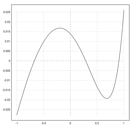
To check this result, we compute the error of (ax+b)/(1+cx)-exp(x). To be able to evaluate the expression, we define a, b, c globally.
>a=v[1]; b=v[2]; c=v[3];
>plot2d("fexpr(x)-exp(x)",-1,1):
The Levenberg-Marquard algorithm leads to the same result.
>nlfit("f","Df",[0,0,1/2])
[0.52432, 1.01388, -0.439515]